
Tutorial de TikZ para principiantes
TikZ es la biblioteca de LaTeX que permite dibujar figuras, grafos y esquemas directamente en su documento, sin software externo. Este tutorial cubre las bases — suficiente para realizar el 90 % de las figuras que necesitarás. Cada ejemplo es compilable directamente en su navegador: haga clic en «Ver en la demo» para ver el resultado al instante, sin instalar LaTeX.
¿Qué es TikZ?
TikZ (acrónimo recursivo: «TikZ ist kein Zeichenprogramm» — TikZ no es un programa de dibujo) es una biblioteca de dibujo vectorial para LaTeX. Está construida sobre el lenguaje PGF y ofrece una sintaxis más accesible.
En concreto: describe su figura con comandos de texto (por ejemplo \draw (0,0) -- (1,1) traza una línea), y TikZ la renderiza en un PDF de calidad profesional. Ideal para esquemas matemáticos, diagramas científicos, organigramas y todo lo que exige precisión.
Para usar TikZ, basta con incluir dos líneas en el preámbulo de su documento:
\documentclass{article}
\usepackage{tikz}

\begin{document}

\begin{tikzpicture}
  % Vos commandes TikZ ici
\end{tikzpicture}

\end{document}
Todos los comandos de dibujo deben escribirse entre \begin{tikzpicture} y \end{tikzpicture}. Es este entorno el que define la zona de dibujo.
\begin{tikzpicture}
  \draw (0,0) -- (3,2);
\end{tikzpicture}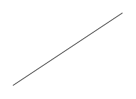
\begin{tikzpicture}
  % Grille de fond (aide visuelle)
  \draw[help lines, gray!30] (0,0) grid (4,3);
  % Quelques points
  \fill[red] (1,1) circle (2pt);
  \fill[blue] (3,2) circle (2pt);
  \fill[green!60!black] (2,0) circle (2pt);
  % Étiquettes
  \node[above right] at (1,1) {(1,1)};
  \node[above right] at (3,2) {(3,2)};
  \node[above right] at (2,0) {(2,0)};
\end{tikzpicture}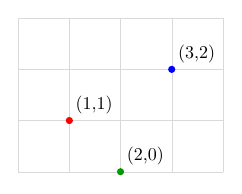
\begin{tikzpicture}
  \draw[red, thick]      (0,2) -- (4,2) node[right] {rouge};
  \draw[blue, thick]     (0,1) -- (4,1) node[right] {bleu};
  \draw[green!60!black, thick] (0,0) -- (4,0) node[right] {vert};
\end{tikzpicture}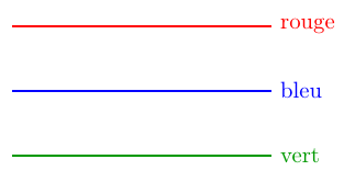
\begin{tikzpicture}
  \draw[thick]                (0,3) -- (4,3) node[right] {trait normal};
  \draw[ultra thick]          (0,2.2) -- (4,2.2) node[right] {ultra thick};
  \draw[dashed, thick]        (0,1.4) -- (4,1.4) node[right] {pointillés};
  \draw[dotted, thick]        (0,0.6) -- (4,0.6) node[right] {points};
  \draw[loosely dashed]       (0,-0.2) -- (4,-0.2) node[right] {loosely dashed};
\end{tikzpicture}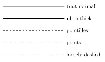
\begin{tikzpicture}
  % Rectangle : (coin bas-gauche) rectangle (coin haut-droit)
  \draw[blue, thick] (0,0) rectangle (3,2);
  % Cercle : (centre) circle (rayon)
  \draw[red, thick] (5,1) circle (1cm);
  % Ellipse : (centre) ellipse (rayon-x and rayon-y)
  \draw[green!60!black, thick] (8,1) ellipse (1.2 and 0.7);
\end{tikzpicture}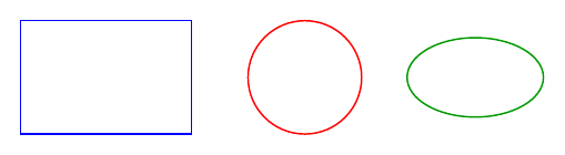
\begin{tikzpicture}
  % Un nœud rectangulaire
  \node[draw, rectangle, fill=blue!10] at (0,0) {Boîte};
  % Un nœud circulaire
  \node[draw, circle, fill=red!10] at (3,0) {Rond};
  % Texte simple sans cadre
  \node at (6,0) {Juste du texte};
\end{tikzpicture}
\usetikzlibrary{positioning}
\begin{tikzpicture}[node distance=10mm and 14mm]
  % Nœud A : position absolue (point d'ancrage)
  \node[draw, rectangle, fill=blue!15, minimum size=10mm] (A) {A};

  % B à droite de A (écart par défaut)
  \node[draw, rectangle, fill=red!15, minimum size=10mm, right=of A] (B) {B};

  % C en dessous de A
  \node[draw, rectangle, fill=green!15, minimum size=10mm, below=of A] (C) {C};

  % D en bas-à-droite de A, distance personnalisée
  \node[draw, rectangle, fill=orange!20, minimum size=10mm,
        below right=15mm and 25mm of A] (D) {D};

  % Ancres : on relie des bords précis (south, north east…)
  \draw[->, thick] (A.south) -- (C.north);
  \draw[->, thick, dashed] (B.south west) -- (D.north);
  \draw[->, thick] (B.east) -- ++(0.6,0) node[right] {(B.east)};
\end{tikzpicture}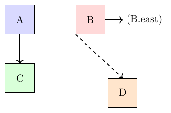
\begin{tikzpicture}
  \draw[->, thick]    (0,3) -- (4,3) node[right] {flèche simple};
  \draw[<-, thick]    (0,2) -- (4,2) node[right] {flèche inverse};
  \draw[<->, thick]   (0,1) -- (4,1) node[right] {bidirectionnelle};
  % Flèche fine personnalisée (bibliothèque arrows.meta)
  \draw[-{Stealth}, very thick, red] (0,0) -- (4,0) node[right] {Stealth};
\end{tikzpicture}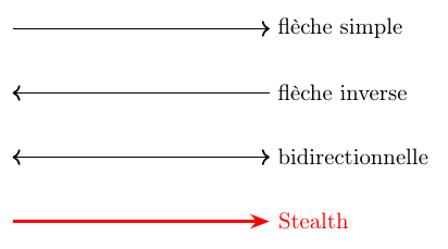
\begin{tikzpicture}
  % Triangle fermé avec 'cycle'
  \draw[blue, thick] (0,0) -- (2,0) -- (1,1.7) -- cycle;
  % Polygone irrégulier
  \draw[red, thick, fill=red!10] (3,0) -- (5,0) -- (5.5,1.5) -- (3.5,2) -- cycle;
\end{tikzpicture}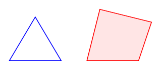
\begin{tikzpicture}
  % Arc de cercle : (départ) arc (angle1:angle2:rayon)
  \draw[blue, thick] (0,0) arc (0:180:1);
  % Courbe de Bézier : (départ) .. controls (P1) and (P2) .. (arrivée)
  \draw[red, thick] (3,0) .. controls (4,2) and (5,-1) .. (6,1);
\end{tikzpicture}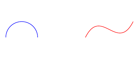
\begin{tikzpicture}
  % Bézier cubique : (A) .. controls (P1) and (P2) .. (B)
  \draw[blue, thick] (0,0) .. controls (1,2) and (3,2) .. (4,0)
    node[right, blue] {Bézier cubique};
  % Points de contrôle visibles
  \fill[blue!50] (1,2) circle (1.5pt) node[above] {\scriptsize $P_1$};
  \fill[blue!50] (3,2) circle (1.5pt) node[above] {\scriptsize $P_2$};
  \draw[blue!50, dashed, thin] (0,0) -- (1,2) -- (3,2) -- (4,0);

  % Bézier quadratique (un seul point de contrôle)
  \draw[red, thick] (0,-2) .. controls (2,-4) .. (4,-2)
    node[right, red] {Bézier quadratique};
  \fill[red!50] (2,-4) circle (1.5pt) node[below] {\scriptsize $P$};
\end{tikzpicture}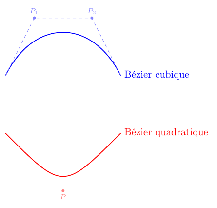
\begin{tikzpicture}
  % \fill remplit (sans contour)
  \fill[blue!30] (0,0) rectangle (2,1.5);
  % \filldraw remplit ET dessine le contour
  \filldraw[red!30, draw=red, thick] (3,0) rectangle (5,1.5);
  % \draw[fill=...] équivalent
  \draw[fill=green!30, thick, green!60!black] (6,0) circle (0.8);
\end{tikzpicture}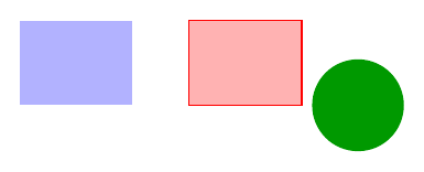
\begin{tikzpicture}
  % Axes
  \draw[->, thick] (-0.5,0) -- (4.5,0) node[right] {$x$};
  \draw[->, thick] (0,-0.5) -- (0,3.5) node[above] {$y$};
  % Graduations
  \foreach \x in {1,2,3,4}
    \draw[gray!50] (\x,-0.05) -- (\x,0.05) node[below=2pt] {\x};
  \foreach \y in {1,2,3}
    \draw[gray!50] (-0.05,\y) -- (0.05,\y) node[left=2pt] {\y};
  % Un point
  \fill[red] (3,2) circle (2pt) node[above right] {A};
\end{tikzpicture}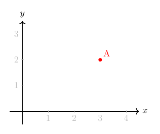
\begin{tikzpicture}[scale=1.2]
  % Axes
  \draw[->, thick] (-3.2,0) -- (3.2,0) node[right] {$x$};
  \draw[->, thick] (0,-1.5) -- (0,4.5) node[above] {$y$};
  % Tracé de y = x²
  \draw[blue, thick, smooth, samples=100, domain=-2:2]
    plot (\x, {\x*\x}) node[right] {$y = x^2$};
\end{tikzpicture}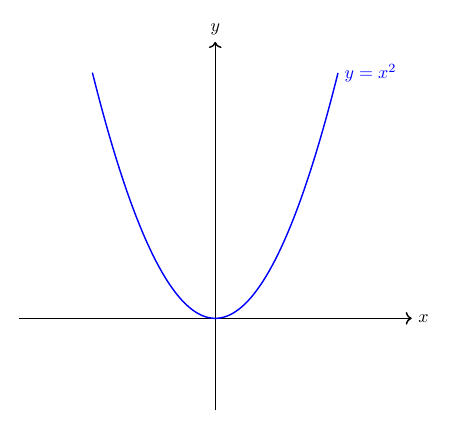
\begin{tikzpicture}[scale=1.2]
  % Axes
  \draw[->, thick] (-3.5,0) -- (3.5,0) node[right] {$x$};
  \draw[->, thick] (0,-2.5) -- (0,2.5) node[above] {$y$};
  % Quelques graduations
  \foreach \x in {-3,-2,-1,1,2,3} \draw (\x, 0.05) -- (\x, -0.05) node[below] {\scriptsize\x};
  % Sinus en bleu
  \draw[blue, thick, smooth, samples=100, domain=-3.14:3.14]
    plot (\x, {sin(\x r)}) node[right] {$\sin x$};
  % Cosinus en rouge
  \draw[red, thick, smooth, samples=100, domain=-3.14:3.14]
    plot (\x, {cos(\x r)}) node[above right] {$\cos x$};
\end{tikzpicture}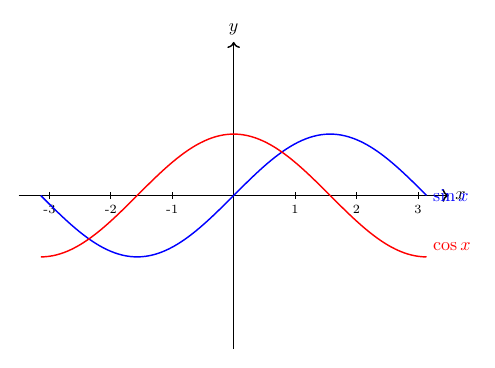
\begin{tikzpicture}[scale=1.0]
  % Axes
  \draw[->, thick] (-0.5,0) -- (5.5,0) node[right] {$x$};
  \draw[->, thick] (0,-0.5) -- (0,3.5) node[above] {$y$};
  % y = sqrt(x) sur [0;5]
  \draw[teal, thick, smooth, samples=80, domain=0:5]
    plot (\x, {sqrt(\x)}) node[right] {$y = \sqrt{x}$};
  % Aire sous la courbe (remplie)
  \fill[teal, opacity=0.2, smooth, samples=80, domain=0:4]
    plot (\x, {sqrt(\x)}) -- (4,0) -- (0,0) -- cycle;
  % Étiquette
  \node[below] at (2, -0.3) {$\int_0^4 \sqrt{x}\,dx$};
\end{tikzpicture}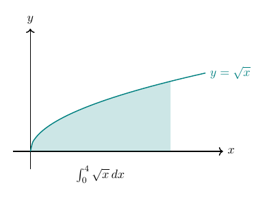
Para ir más allá
Ahora dominas los fundamentos. Para pasar al siguiente nivel:
- Galería TikZ: más de 300 figuras clasificadas por categoría (matemáticas, física, química, machine learning, diagramas…). Haga clic en cualquier figura para ver el código completo y editarlo en la demo.
- pgfplots para los gráficos de funciones y las estadísticas:
\usepackage{pgfplots}. - tikz-cd para los diagramas conmutativos en matemáticas.
- circuitikz para los esquemas eléctricos.
- Las bibliotecas TikZ útiles para cargar:
arrows.meta,positioning,calc,decorations.markings,patterns.