TikZ Tutorial for Beginners

What is TikZ?

TikZ (a recursive acronym for « TikZ ist kein Zeichenprogramm » — TikZ is not a drawing program) is a vector drawing library for LaTeX, built on top of the PGF language with a friendlier syntax.

Concretely: you describe your figure with text commands (for example \draw (0,0) -- (1,1) draws a line), and TikZ renders it as a professional-quality PDF. Perfect for mathematical schematics, scientific diagrams, flowcharts, and anything that demands precision.

To use TikZ, just include two lines in your document preamble:

\documentclass{article}
\usepackage{tikz}

\begin{document}

\begin{tikzpicture}
  % Vos commandes TikZ ici
\end{tikzpicture}

\end{document}

All drawing commands must be written between \begin{tikzpicture} and \end{tikzpicture}. This environment defines the drawing area.

First drawing: a line

The basic TikZ command is \draw. To draw a line, give two points joined by --.

Coordinates are written in parentheses as (x,y); the default unit is centimetres. (0,0) is the origin, (3,2) is 3 cm to the right and 2 cm above.

\begin{tikzpicture}
  \draw (0,0) -- (3,2);
\end{tikzpicture}

Coordinates and points

To see where you're drawing, it helps to display a reference grid with \draw[help lines] (0,0) grid (4,3);.

You can mark a point by filling a small circle with \fill, and label its position with a \node (see the dedicated chapter below).

\begin{tikzpicture}
  % Background grid (visual aid)
  \draw[help lines, gray!30] (0,0) grid (4,3);
  % A few points
  \fill[red] (1,1) circle (2pt);
  \fill[blue] (3,2) circle (2pt);
  \fill[green!60!black] (2,0) circle (2pt);
  % Labels
  \node[above right] at (1,1) {(1,1)};
  \node[above right] at (3,2) {(3,2)};
  \node[above right] at (2,0) {(2,0)};
\end{tikzpicture}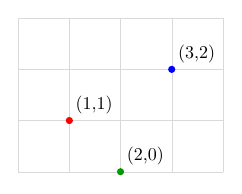

Colors

TikZ accepts predefined colors: red, blue, green, black, white, gray, orange, purple, etc.

You can also tune the intensity with !: red!50 is 50 % red (lighter), green!60!black mixes 60 % green and 40 % black (dark green).

Apply a color via the square-bracket options of \draw.

\begin{tikzpicture}
  \draw[red, thick]      (0,2) -- (4,2) node[right] {red};
  \draw[blue, thick]     (0,1) -- (4,1) node[right] {blue};
  \draw[green!60!black, thick] (0,0) -- (4,0) node[right] {green};
\end{tikzpicture}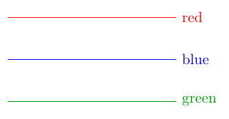

Line styles

Line thickness is set with thin, thick, very thick, ultra thick, or with line width=1pt for an exact value.

Line pattern is set with dashed, dotted, loosely dashed, densely dotted, etc.

\begin{tikzpicture}
  \draw[thick]                (0,3) -- (4,3) node[right] {normal line};
  \draw[ultra thick]          (0,2.2) -- (4,2.2) node[right] {ultra thick};
  \draw[dashed, thick]        (0,1.4) -- (4,1.4) node[right] {dashed};
  \draw[dotted, thick]        (0,0.6) -- (4,0.6) node[right] {dotted};
  \draw[loosely dashed]       (0,-0.2) -- (4,-0.2) node[right] {loosely dashed};
\end{tikzpicture}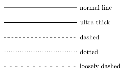

Rectangle, circle, ellipse

A rectangle is drawn with (corner1) rectangle (corner2), where corner1 and corner2 are two opposite corners (typically bottom-left and top-right).

A circle is drawn with (center) circle (radius).

An ellipse needs two radii (horizontal and vertical): (center) ellipse (rx and ry).

\begin{tikzpicture}
  % Rectangle: (bottom-left corner) rectangle (top-right corner)
  \draw[blue, thick] (0,0) rectangle (3,2);
  % Circle: (center) circle (radius)
  \draw[red, thick] (5,1) circle (1cm);
  % Ellipse: (center) ellipse (x-radius and y-radius)
  \draw[green!60!black, thick] (8,1) ellipse (1.2 and 0.7);
\end{tikzpicture}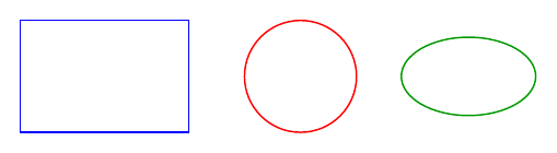

Nodes and text

A node is a positionable object containing text or shapes. The basic command is \node at (x,y) {content};.

With options, the node can be framed: draw (draw the outline), rectangle or circle (shape), fill=blue!10 (background color).

\begin{tikzpicture}
  % A rectangular node
  \node[draw, rectangle, fill=blue!10] at (0,0) {Box};
  % A circular node
  \node[draw, circle, fill=red!10] at (3,0) {Round};
  % Plain text, no frame
  \node at (6,0) {Just text};
\end{tikzpicture}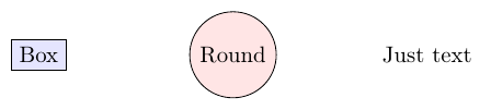

Positioning nodes (right=of, below=of…)

Computing each node's coordinates by hand quickly becomes tedious. The positioning library lets you place a node relative to another: right=of A places the node to the right of A, below=of A below it, etc. To use it, add \usetikzlibrary{positioning} to the preamble.

Available directions: right, left, above, below and their combinations (above right, below left…). You can specify a distance: below=2cm of A, or globally with node distance=15mm as an option of the tikzpicture.

Each node also has named anchors (north, south, east, west, north east, center…). Access them with the syntax (A.south) — this is essential to connect two nodes cleanly: \draw (A.east) -- (B.west); draws an arrow between edges without crossing them.

Tip: naming a node with (A) right after \node is mandatory if you want to reference it later: \node[draw] (A) at (0,0) {Text};.

\usetikzlibrary{positioning}
\begin{tikzpicture}[node distance=10mm and 14mm]
  % Node A: absolute position (anchor point)
  \node[draw, rectangle, fill=blue!15, minimum size=10mm] (A) {A};

  % B to the right of A (default spacing)
  \node[draw, rectangle, fill=red!15, minimum size=10mm, right=of A] (B) {B};

  % C below A
  \node[draw, rectangle, fill=green!15, minimum size=10mm, below=of A] (C) {C};

  % D below-right of A, custom distance
  \node[draw, rectangle, fill=orange!20, minimum size=10mm,
        below right=15mm and 25mm of A] (D) {D};

  % Anchors: connect specific edges (south, north east…)
  \draw[->, thick] (A.south) -- (C.north);
  \draw[->, thick, dashed] (B.south west) -- (D.north);
  \draw[->, thick] (B.east) -- ++(0.6,0) node[right] {(B.east)};
\end{tikzpicture}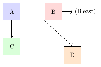

Arrows

Arrows are obtained by adding tip options: -> (forward arrow), <- (reverse arrow), <-> (bidirectional).

For nicer arrowheads, load the arrows.meta library in the preamble: \usetikzlibrary{arrows.meta}. You can then use -{Stealth}, -{Latex}, -{Triangle}, etc.

\begin{tikzpicture}
  \draw[->, thick]    (0,3) -- (4,3) node[right] {forward arrow};
  \draw[<-, thick]    (0,2) -- (4,2) node[right] {reverse arrow};
  \draw[<->, thick]   (0,1) -- (4,1) node[right] {bidirectional};
  % Custom thin arrowhead (arrows.meta library)
  \draw[-{Stealth}, very thick, red] (0,0) -- (4,0) node[right] {Stealth};
\end{tikzpicture}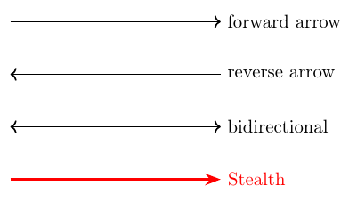

Polygons and closed paths

To draw a polygon, chain several -- segments and end with -- cycle, which closes the path cleanly.

To fill it (in addition to the outline), use the fill=color option inside \draw.

\begin{tikzpicture}
  % Closed triangle with 'cycle'
  \draw[blue, thick] (0,0) -- (2,0) -- (1,1.7) -- cycle;
  % Irregular polygon
  \draw[red, thick, fill=red!10] (3,0) -- (5,0) -- (5.5,1.5) -- (3.5,2) -- cycle;
\end{tikzpicture}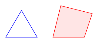

Arcs and curves

A circular arc is drawn with (start) arc (startAngle:endAngle:radius). Angles are in degrees.

For smooth curves, use Bézier curves (next chapter).

\begin{tikzpicture}
  % Circular arc: (start) arc (angle1:angle2:radius)
  \draw[blue, thick] (0,0) arc (0:180:1);
  % Bézier curve: (start) .. controls (P1) and (P2) .. (end)
  \draw[red, thick] (3,0) .. controls (4,2) and (5,-1) .. (6,1);
\end{tikzpicture}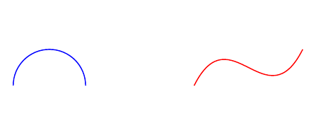

Bézier curves

A cubic Bézier curve is drawn with (A) .. controls (P1) and (P2) .. (B). The path starts at A, ends at B, and is guided by two control points P1 and P2 — the curve doesn't have to pass through them, they pull the curve like magnets.

A quadratic Bézier uses a single control point: (A) .. controls (P) .. (B). Easier to tune when you want a symmetric curve.

Teaching tip: drawing the control points with \fill plus their control polygon as dashed lines greatly helps students see how the curve is built.

\begin{tikzpicture}
  % Cubic Bézier: (A) .. controls (P1) and (P2) .. (B)
  \draw[blue, thick] (0,0) .. controls (1,2) and (3,2) .. (4,0)
    node[right, blue] {cubic Bézier};
  % Visible control points
  \fill[blue!50] (1,2) circle (1.5pt) node[above] {\scriptsize $P_1$};
  \fill[blue!50] (3,2) circle (1.5pt) node[above] {\scriptsize $P_2$};
  \draw[blue!50, dashed, thin] (0,0) -- (1,2) -- (3,2) -- (4,0);

  % Quadratic Bézier (single control point)
  \draw[red, thick] (0,-2) .. controls (2,-4) .. (4,-2)
    node[right, red] {quadratic Bézier};
  \fill[red!50] (2,-4) circle (1.5pt) node[below] {\scriptsize $P$};
\end{tikzpicture}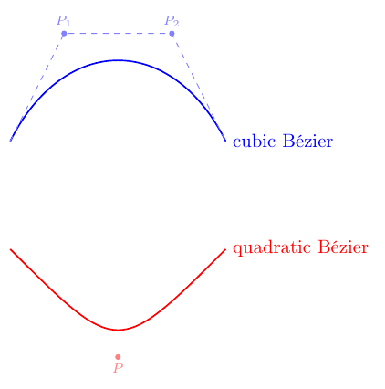

Filling

To fill a shape without an outline, use \fill. To fill with an outline, use \filldraw, or add the fill=... option to your \draw.

You can also apply opacity with fill opacity=0.3 for semi-transparent overlays.

\begin{tikzpicture}
  % \fill fills (no outline)
  \fill[blue!30] (0,0) rectangle (2,1.5);
  % \filldraw fills AND draws the outline
  \filldraw[red!30, draw=red, thick] (3,0) rectangle (5,1.5);
  % \draw[fill=...] equivalent
  \draw[fill=green!30, thick, green!60!black] (6,0) circle (0.8);
\end{tikzpicture}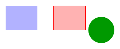

Axes and grid

For a simple orthonormal frame, use two \draw[->] with a \node at the end to label the axis.

The \foreach \x in {1,2,3,4} construct repeats a drawing for each value — handy for tick marks.

\begin{tikzpicture}
  % Axes
  \draw[->, thick] (-0.5,0) -- (4.5,0) node[right] {$x$};
  \draw[->, thick] (0,-0.5) -- (0,3.5) node[above] {$y$};
  % Tick marks
  \foreach \x in {1,2,3,4}
    \draw[gray!50] (\x,-0.05) -- (\x,0.05) node[below=2pt] {\x};
  \foreach \y in {1,2,3}
    \draw[gray!50] (-0.05,\y) -- (0.05,\y) node[left=2pt] {\y};
  % A point
  \fill[red] (3,2) circle (2pt) node[above right] {A};
\end{tikzpicture}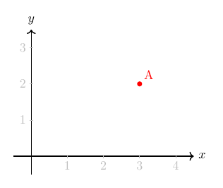

Plotting a function

To plot a function's graph, use \draw plot (\x, {expression}), where \x is the variable and the math expression goes in braces.

Three essential options: domain=a:b sets the plotting interval, samples=N controls the number of points (more = smoother), and smooth requests smooth interpolation.

This syntax uses pure TikZ, no pgfplots. Perfect for most school-level graphs.

\begin{tikzpicture}[scale=1.2]
  % Axes
  \draw[->, thick] (-3.2,0) -- (3.2,0) node[right] {$x$};
  \draw[->, thick] (0,-1.5) -- (0,4.5) node[above] {$y$};
  % Plot of y = x²
  \draw[blue, thick, smooth, samples=100, domain=-2:2]
    plot (\x, {\x*\x}) node[right] {$y = x^2$};
\end{tikzpicture}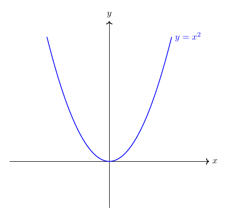

Multiple functions on the same plot

To overlay multiple curves, just repeat \draw plot as many times as needed, varying colors and expressions.

Important for trig functions: TikZ works in degrees by default. To use radians (with π), add r after the argument: sin(\x r).

\begin{tikzpicture}[scale=1.2]
  % Axes
  \draw[->, thick] (-3.5,0) -- (3.5,0) node[right] {$x$};
  \draw[->, thick] (0,-2.5) -- (0,2.5) node[above] {$y$};
  % A few tick marks
  \foreach \x in {-3,-2,-1,1,2,3} \draw (\x, 0.05) -- (\x, -0.05) node[below] {\scriptsize\x};
  % Sine in blue
  \draw[blue, thick, smooth, samples=100, domain=-3.14:3.14]
    plot (\x, {sin(\x r)}) node[right] {$\sin x$};
  % Cosine in red
  \draw[red, thick, smooth, samples=100, domain=-3.14:3.14]
    plot (\x, {cos(\x r)}) node[above right] {$\cos x$};
\end{tikzpicture}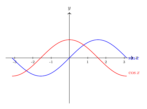

Area under a curve

To render the area under a curve (typically to illustrate an integral), combine \fill with a plot and close the region via -- cycle, passing through the axis edges.

The opacity=0.2 option makes the fill semi-transparent, so the curve stays visible on top.

For more advanced graphs (annotated axes, automatic legend, log scales, statistics), explore the pgfplots package in our gallery.

\begin{tikzpicture}[scale=1.0]
  % Axes
  \draw[->, thick] (-0.5,0) -- (5.5,0) node[right] {$x$};
  \draw[->, thick] (0,-0.5) -- (0,3.5) node[above] {$y$};
  % y = sqrt(x) on [0;5]
  \draw[teal, thick, smooth, samples=80, domain=0:5]
    plot (\x, {sqrt(\x)}) node[right] {$y = \sqrt{x}$};
  % Area under the curve (filled)
  \fill[teal, opacity=0.2, smooth, samples=80, domain=0:4]
    plot (\x, {sqrt(\x)}) -- (4,0) -- (0,0) -- cycle;
  % Label
  \node[below] at (2, -0.3) {$\int_0^4 \sqrt{x}\,dx$};
\end{tikzpicture}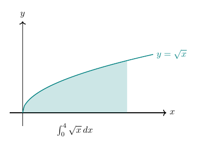

Going further

You now know the fundamentals. To take it to the next level:

• TikZ Gallery: 300+ figures organised by category (mathematics, physics, chemistry, machine learning, diagrams…). Click any figure to see the full code and edit it in the demo.
• pgfplots for function graphs and statistics: \usepackage{pgfplots}.
• tikz-cd for commutative diagrams in mathematics.
• circuitikz for electrical schematics.
• Useful TikZ libraries to load: arrows.meta, positioning, calc, decorations.markings, patterns.